Practical Introduction to Deep Learning with PyTorch

A few weeks ago, I was having a chat with my friend when he asked me to teach him Deep Learning in the simplest way possible. The first step was defining what Deep Learning is, so I wrote an article on Deep Learning in a comical style, and he enjoyed it greatly, you can read this article here. Now, he has requested that I teach practical Deep Learning. In this article, I will attempt to explain Deep Learning in a straightforward manner. So, here is the plan of action:

1. Setting up Environment
2. Introduction to the Dataset: MNIST
3. Lets see some examples
4. Building a Simple Neural Network
5. Training the Model
6. Evaluating the Model
7. View Results
8. Conclusion and Next Steps

Setting Up the Environment

Python and IDEs
Python is the preferred language for deep learning due to its simplicity and extensive library support. Install Python and choose an Integrated Development Environment (IDE) such as Jupyter Notebook for an interactive coding experience.

PyTorch Installation
PyTorch is known for its flexibility and dynamic computation graph that aligns with the way programmers think. Install PyTorch by visiting PyTorch’s official website() and selecting the appropriate installation command for your system or you can just use google colab

Introduction to the Dataset: MNIST

The MNIST dataset, containing 70,000 handwritten digits, is a beginner-friendly dataset used for classification tasks.

import torch 
from torchvision import datasets, transforms 
 
# Define a transform to normalize the data 
transform = transforms.Compose([transforms.ToTensor(), transforms.Normalize((0.5,), (0.5,))]) 
 
# Download and load the training data 
trainset = datasets.MNIST('~/.pytorch/MNIST_data/', download=True, train=True, transform=transform) 
trainloader = torch.utils.data.DataLoader(trainset, batch_size=64, shuffle=True)

Lets see some examples

import matplotlib.pyplot as plt 
 
# Get a batch of images from the trainloader 
dataiter = iter(trainloader) 
images, labels = next(dataiter) 
 
# Display a few images from the batch 
fig, axes = plt.subplots(figsize=(10, 2), ncols=8) 
for i in range(8): 
    ax = axes[i] 
    ax.imshow(images[i].numpy().squeeze(), cmap='gray') 
    ax.axis('off') 
    ax.set_title(f'Label: {labels[i].item()}') 
 
plt.show()

Building a Simple Neural Network

Model Architecture
We will define a simple neural network with one hidden layer.

from torch import nn, optim 
 
# Define the network architecture 
class Network(nn.Module): 
    def __init__(self): 
        super(Network, self).__init__() 
        self.hidden = nn.Linear(784, 256) 
        self.output = nn.Linear(256, 10) 
        self.sigmoid = nn.Sigmoid() 
        self.softmax = nn.Softmax(dim=1) 
         
    def forward(self, x): 
        x = self.hidden(x) 
        x = self.sigmoid(x) 
        x = self.output(x) 
        x = self.softmax(x) 
        return x 
 
model = Network()

further you can see the model layers:

from torchsummary import summary 
 
# Assuming your model is already defined as 'model' 
summary(model, (784,))

---------------------------------------------------------------- 
        Layer (type)               Output Shape         Param # 
================================================================ 
            Linear-1                  [-1, 256]         200,960 
           Sigmoid-2                  [-1, 256]               0 
            Linear-3                   [-1, 10]           2,570 
           Softmax-4                   [-1, 10]               0 
================================================================ 
Total params: 203,530 
Trainable params: 203,530 
Non-trainable params: 0 
---------------------------------------------------------------- 
Input size (MB): 0.00 
Forward/backward pass size (MB): 0.00 
Params size (MB): 0.78 
Estimated Total Size (MB): 0.78 
----------------------------------------------------------------

Compiling the Model
In PyTorch, we define a loss function and an optimizer separately.

# Define the loss 
criterion = nn.CrossEntropyLoss() 
 
# Optimizers require the parameters to optimize and a learning rate 
optimizer = optim.SGD(model.parameters(), lr=0.01)

Training the Model

The training process involves multiple epochs over the training data.

epochs = 5 
for e in range(epochs): 
    running_loss = 0 
    for images, labels in trainloader: 
        # Flatten MNIST images into a 784 long vector 
        images = images.view(images.shape[0], -1) 
     
        # Training pass 
        optimizer.zero_grad() 
         
        output = model(images) 
        loss = criterion(output, labels) 
         
        # Backward pass 
        loss.backward() 
        optimizer.step() 
         
        running_loss += loss.item() 
    else: 
        print(f"Training loss: {running_loss/len(trainloader)}")

Evaluating the Model

After training, evaluate the model performance on test data.

%matplotlib inline 
import helper 
 
images, labels = next(iter(trainloader)) 
 
img = images[0].view(1, 784) 
# Turn off gradients to speed up this part 
with torch.no_grad(): 
    logps = model(img) 
 
# Output of the network are log-probabilities, need to take exponential for probabilities 
ps = torch.exp(logps) 
helper.view_classify(img.view(1, 28, 28), ps)

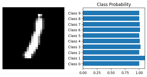
View Results

Let’s visualize the results:

import matplotlib.pyplot as plt 
import numpy as np 
 
def view_classify(image, probabilities, label_names=None): 
    # Convert image tensor to NumPy array 
    image = image.view(1, 28, 28).numpy() 
     
    fig, (ax1, ax2) = plt.subplots(figsize=(6, 9), ncols=2) 
    ax1.imshow(image[0], cmap='gray') 
    ax1.axis('off') 
     
    if label_names is not None: 
        ax2.barh(np.arange(10), probabilities[0]) 
        ax2.set_aspect(0.1) 
        ax2.set_yticks(np.arange(10)) 
         
        if label_names is not None: 
            ax2.set_yticklabels(label_names) 
         
        ax2.set_title('Class Probability') 
        ax2.set_xlim(0, 1.1) 
     
    plt.tight_layout() 
 
# Usage: 
# Call view_classify(img, ps, label_names) where img is your image tensor and ps are the probabilities. 
# label_names is an optional argument for providing class labels.

# After obtaining 'img' and 'ps' 
view_classify(img.view(1, 28, 28), ps, label_names=["Class 0", "Class 1", "Class 2", "Class 3", "Class 4", "Class 5", "Class 6", "Class 7", "Class 8", "Class 9"])

Conclusion and Next Steps

This guide provided an overview of setting up a deep learning environment with PyTorch, working with the MNIST dataset, building a basic neural network, and training it.

So you see how it works, here we used just one hidden layer of DNN so obviously the accuracy will not be great. So in order to get better accuracy we will move towards CNN (convolutional neural network). In next chapter we will learn deeply about how CNN works in detail.

Enjoy 😄