Classification using Random Forest
Learn supervised learning with Random Forest using the iris dataset. This tutorial covers data preprocessing, model training, and results visualization using Python.


How to run code in this article
Hi, today we will learn about supervised learning using Random Forest we will also practically play with iris dataset. . Below, I'll break down the tutorial into several sections:
- Supervised Learning
- Dataset
- Preprocessing
- Model and Training
- Results
1. Supervised Learning
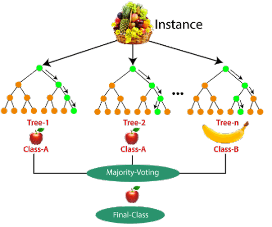
Supervised learning is a type of machine learning where the model is trained on a labeled dataset. The dataset consists of input-output pairs, and the goal is for the model to learn to map inputs to outputs. This training allows the model to make predictions or decisions without being explicitly programmed to perform the task. In this article we will classify dataset using Random forest model. Random forest is a machine learning method that creates many decision trees and combines their results to make better predictions. This approach improves accuracy and reduces errors by averaging the outcomes of multiple trees (see the example below).
2. Dataset
Download Dataset
First step is download the dataset, you can either download the dataset from the link below or download it from kaggle. I have inserted the data here just for ease.
Now lets open the Colab IDE (integrated development environment) and import the relevant libraries.
Load and Visualize Dataset
First import all libraries:
# import seaborn, pandas and sklearn libraries
import seaborn as sns
import pandas as pd
from sklearn.model_selection import train_test_split
from sklearn.linear_model import LinearRegression
from sklearn.metrics import mean_squared_error
from sklearn.preprocessing import StandardScaler
from sklearn.pipeline import Pipeline
from sklearn.model_selection import cross_val_score
from sklearn.model_selection import KFold
from sklearn.preprocessing import PolynomialFeatures
import matplotlib.pyplot as plt
import libraries
Data visualization, now we use seaborn libraries to understand the csv file structure.
df = pd.read_csv('iris.csv', index_col=0)
df.head(4)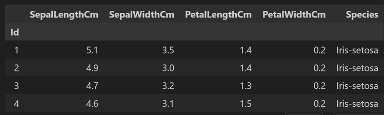
Now lets visualize the columns of the dataset using pairplot
sns.set_style("whitegrid")
sns.pairplot(df,hue="Species",size=3);
plt.show()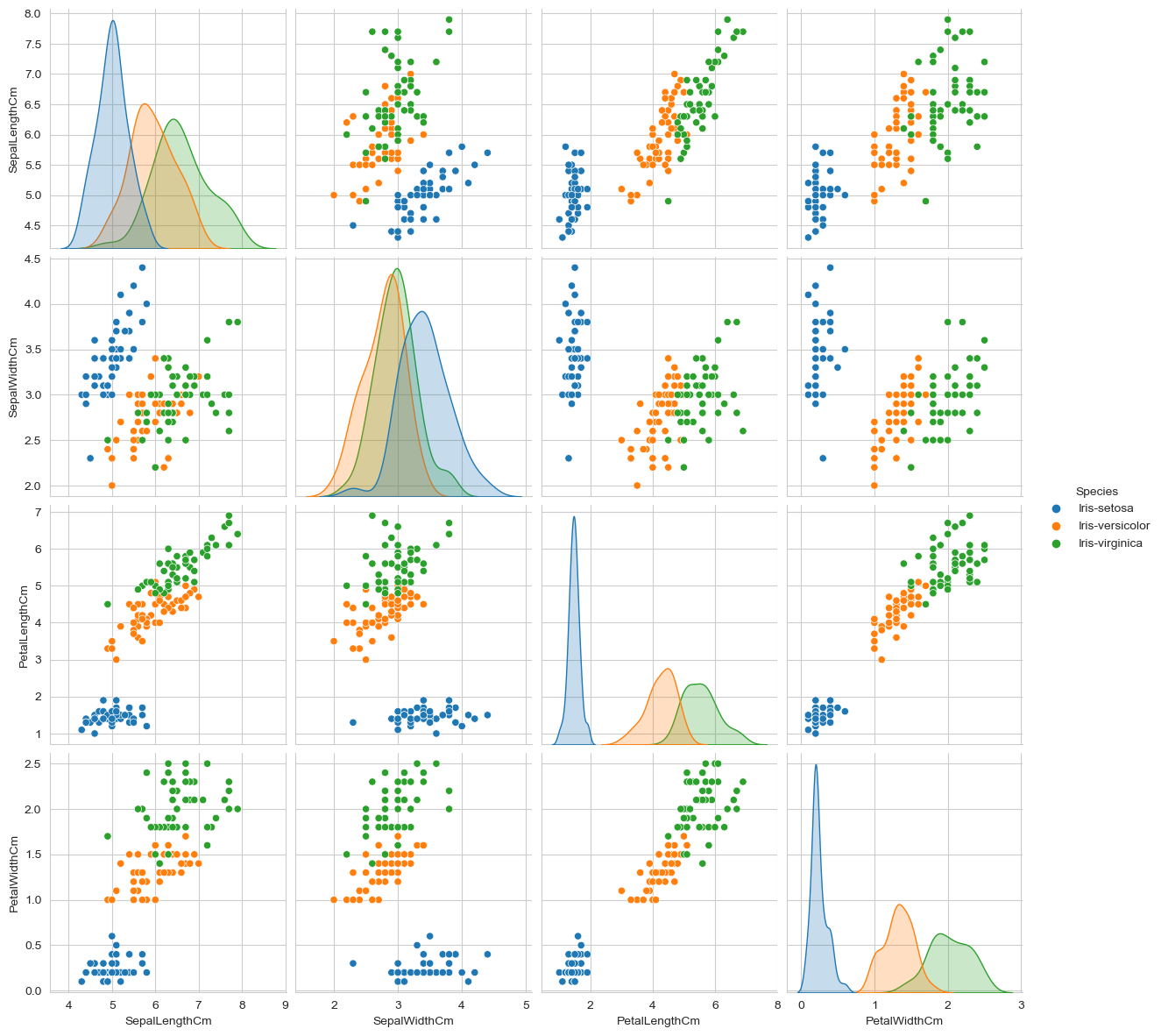
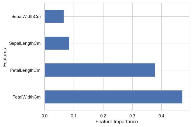
Feature Importance
There is a lot in terms of visualization (please check the google colab file), lets use plotly for feature importance. This plot shows which feature is important for classification model. Here 'PetalWidthCm' has highest importance.
from sklearn.ensemble import ExtraTreesClassifier

# Assume df is already loaded with your data
X = df.drop(['Species', 'Id'], axis=1)  # features
y = df['Species']  # target

# Feature selection using Extra Trees Classifier
feat_selection = ExtraTreesClassifier()
feat_selection.fit(X, y)
feat_importances = pd.Series(feat_selection.feature_importances_, index=X.columns)

# Sorting features by importance
sorted_importances = feat_importances.sort_values(ascending=True)

# Creating a bar plot for feature importances
fig = px.bar(sorted_importances,
             orientation='h',
             labels={'value': 'Feature Importance', 'index': 'Features'},
             title='Feature Importance Ranking',
             color=sorted_importances.values,
             color_continuous_scale='Viridis')

# Enhancing the layout
fig.update_layout(xaxis_title='Feature Importance',
                  yaxis_title='Features',
                  coloraxis_showscale=False, # Turn off color scale if not needed
                  plot_bgcolor='white')

# Display the plot
fig.show()
Get the feature importance
3. Preprocessing
This process can have multiple steps depending on the task, this dataset is well filtered and maintained so we can skip the those steps for now, we will discuss them later in other articles. For now we will only divide the dataset into train test and validation set.
# divide the dataset into the training, test and validation sets
X_train, X_test, y_train, y_test = train_test_split(X, y, test_size=0.2, random_state=42)
X_train, X_val, y_train, y_val = train_test_split(X_train, y_train, test_size=0.2, random_state=42)

# print the shape of the training, test and validation sets
print(X_train.shape, X_test.shape, X_val.shape)
Divide the dataset into train validation and test set
4. Model and Training
Now lets prepare the model and train it on different parameters.
# make a random forest classifier model and train validat the model and finally test it
from sklearn.ensemble import RandomForestClassifier
from sklearn.metrics import accuracy_score

est = [5, 10, 15, 20, 25, 30, 35, 40, 45, 50, 60, 70, 80, 90, 100]
train_accuracy_ = []
val_accuracy_ = []
test_accuracy_ = []

for i in range(len(est)):

    # create a random forest classifier model
    rf = RandomForestClassifier(n_estimators=est[i], random_state=42)

    # train the model
    rf.fit(X_train, y_train)

    # test the model in trainign set
    y_train_pred = rf.predict(X_train)
    train_accuracy = accuracy_score(y_train, y_train_pred)
    print(f'Training accuracy: {train_accuracy}')
    train_accuracy_.append(train_accuracy)

    # validate the model
    y_val_pred = rf.predict(X_val)
    val_accuracy = accuracy_score(y_val, y_val_pred)
    print(f'Validation accuracy: {val_accuracy}')
    val_accuracy_.append(val_accuracy)

    # test the model
    y_test_pred = rf.predict(X_test)
    test_accuracy = accuracy_score(y_test, y_test_pred)
    print(f'Test accuracy: {test_accuracy}')
    test_accuracy_.append(test_accuracy)


# plot the training, validation and test accuracies with respect to the number of estimators
plt.figure(figsize=(10, 6))
plt.plot(est, train_accuracy_, '-o', label='Training Accuracy')
plt.plot(est, val_accuracy_, '-o', label='Validation Accuracy')
plt.plot(est, test_accuracy_, '-o', label='Test Accuracy')
plt.xticks(est)
plt.xlabel('Number of Estimators')
plt.ylabel('Accuracy')
plt.title('Random Forest Classifier Accuracy')
plt.legend()
plt.show()
Model and Training
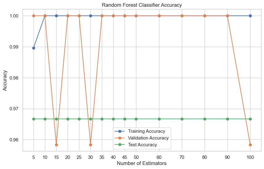
What did you notice ? all of them has almost same training and testing accuracy (green line). So choose any model you want (with number of estimators 10, 20, 25, and 35-90) because validation accuracy is highest in all them with training accuracy.
5. Results
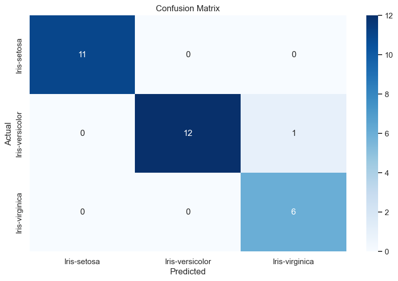
In order to visualize the the results we use confusion matrix. A confusion matrix is a table that summarizes the performance of a classification model by showing the counts of true positives, true negatives, false positives, and false negatives. It helps evaluate how well the model distinguishes between different classes.
from sklearn.metrics import confusion_matrix
cm = confusion_matrix(y_test, y_test_pred, labels=['Iris-setosa', 'Iris-versicolor', 'Iris-virginica'])
plt.figure(figsize=(10, 6))
sns.heatmap(cm, annot=True, fmt='d', cmap='Blues', xticklabels=['Iris-setosa', 'Iris-versicolor', 'Iris-virginica'], yticklabels=['Iris-setosa', 'Iris-versicolor', 'Iris-virginica'])
plt.xlabel('Predicted')
plt.ylabel('Actual')
plt.title('Confusion Matrix')
plt.show()
Confusion Matrix
Finally get classification report from sklearn library
# get the report of the model
from sklearn.metrics import classification_report
report = classification_report(y_test, y_test_pred)
print(report)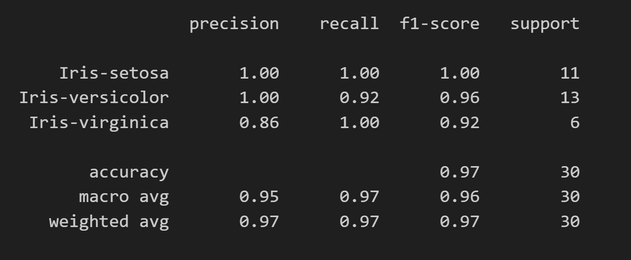
It is amazing right, enjoy the article, I will see you again 😄