DINOv2 for Custom Dataset Segmentation: A Comprehensive Tutorial.
Discover DINOv2, a powerful self-supervised vision transformer trained on 142M images. This tutorial guides you through data loading, preprocessing, model definition, and training using PyTorch.

After YOLOv8 and SAM (Segment Anything Model), the most anticipated computer vision model is DINOv2. I got the motivation for this tutorial from this GitHub repository: https://github.com/NielsRogge/Transformers-Tutorials/tree/master, while running the code, I found 2 bugs because of that, I got some annoying errors while training the model (in his tutorial, he stopped the training the process after some steps and error arises in between and at last training step). The entire code is taken from his notebook (except for some changes :) ), and here is the plan of attack:
Plan of Attack
- Introduction of DINOv2
- Library installation
- Load dataset
- Create PyTorch dataset
- Create PyTorch dataloaders
- Define model
- Train the model
Introduction of DINOv2
DINOv2 is a vision transformer that has been trained in a self-supervised manner on a meticulously curated dataset of 142 million images. It offers the best image features, or embeddings, available for downstream tasks such as image classification, image segmentation, and depth estimation.
Figure 1 conceptualizes this approach, in this tutorial, I am simply training a linear transformation (1*1 CNN layer) on top of a frozen DINOv2 backbone. This transformation will map the features (patch embeddings) to logits (the unnormalized scores output by neural networks, indicative of the model’s predictions). In the context of semantic segmentation, the logits will take the shape of (batch_size, num_classes, height, and width), corresponding to a predicted class for each pixel.
Library installation
Here are two main libraries:
!pip install -q git+https://github.com/huggingface/transformers.git datasets

!pip install -q evaluate
Load dataset
Next, let’s load an image segmentation dataset. In this case, we’ll use the Foodseg dataset.
from datasets import load_dataset

#dataset
dataset = load_dataset("EduardoPacheco/FoodSeg103")

#lables
id2label = {
    0: "background",
    1: "candy",
    2: "egg tart",
    3: "french fries",
    4: "chocolate",
    5: "biscuit",
    6: "popcorn",
    7: "pudding",
    8: "ice cream",
    9: "cheese butter",
    10: "cake",
    11: "wine",
    12: "milkshake",
    13: "coffee",
    14: "juice",
    15: "milk",
    16: "tea",
    17: "almond",
    18: "red beans",
    19: "cashew",
    20: "dried cranberries",
    21: "soy",
    22: "walnut",
    23: "peanut",
    24: "egg",
    25: "apple",
    26: "date",
    27: "apricot",
    28: "avocado",
    29: "banana",
    30: "strawberry",
    31: "cherry",
    32: "blueberry",
    33: "raspberry",
    34: "mango",
    35: "olives",
    36: "peach",
    37: "lemon",
    38: "pear",
    39: "fig",
    40: "pineapple",
    41: "grape",
    42: "kiwi",
    43: "melon",
    44: "orange",
    45: "watermelon",
    46: "steak",
    47: "pork",
    48: "chicken duck",
    49: "sausage",
    50: "fried meat",
    51: "lamb",
    52: "sauce",
    53: "crab",
    54: "fish",
    55: "shellfish",
    56: "shrimp",
    57: "soup",
    58: "bread",
    59: "corn",
    60: "hamburg",
    61: "pizza",
    62: "hanamaki baozi",
    63: "wonton dumplings",
    64: "pasta",
    65: "noodles",
    66: "rice",
    67: "pie",
    68: "tofu",
    69: "eggplant",
    70: "potato",
    71: "garlic",
    72: "cauliflower",
    73: "tomato",
    74: "kelp",
    75: "seaweed",
    76: "spring onion",
    77: "rape",
    78: "ginger",
    79: "okra",
    80: "lettuce",
    81: "pumpkin",
    82: "cucumber",
    83: "white radish",
    84: "carrot",
    85: "asparagus",
    86: "bamboo shoots",
    87: "broccoli",
    88: "celery stick",
    89: "cilantro mint",
    90: "snow peas",
    91: "cabbage",
    92: "bean sprouts",
    93: "onion",
    94: "pepper",
    95: "green beans",
    96: "French beans",
    97: "king oyster mushroom",
    98: "shiitake",
    99: "enoki mushroom",
    100: "oyster mushroom",
    101: "white button mushroom",
    102: "salad",
    103: "other ingredients"
}

# visualize the images and masks
import numpy as np
import matplotlib.pyplot as plt

# map every class to a random color
id2color = {k: list(np.random.choice(range(256), size=3)) for k,v in id2label.items()}

def visualize_map(image, segmentation_map):
    color_seg = np.zeros((segmentation_map.shape[0], segmentation_map.shape[1], 3), dtype=np.uint8) # height, width, 3
    for label, color in id2color.items():
        color_seg[segmentation_map == label, :] = color

    # Show image + mask
    img = np.array(image) * 0.5 + color_seg * 0.5
    img = img.astype(np.uint8)

    plt.figure(figsize=(15, 10))
    plt.imshow(img)
    plt.show()

visualize_map(image, segmentation_map)
Create PyTorch dataset
To prepare examples for the model, we create a standard PyTorch dataset that includes image augmentations. We randomly resize and crop the training images to a uniform resolution of 448x448 pixels and normalize the color channels, ensuring all training images are of the same fixed resolution. For this process, we employ the Albumentations library, although it’s worth noting that other libraries, such as Torchvision or Kornia, can also serve this purpose.
It’s important to remember that the model expects input pixel_values with the shape (batch_size, num_channels, height, width). Since Albumentations operates on NumPy arrays, which use a channels-last format, we need to reorder the dimensions to place the channels first. In addition, the model requires labels in the shape of (batch_size, height, and width), which provide the ground truth label for each pixel in every example of the batch.
from torch.utils.data import Dataset
import torch

class SegmentationDataset(Dataset):
  def __init__(self, dataset, transform):
    self.dataset = dataset
    self.transform = transform

  def __len__(self):
    return len(self.dataset)

  def __getitem__(self, idx):
    item = self.dataset[idx]
    original_image = np.array(item["image"])
    original_segmentation_map = np.array(item["label"])

    transformed = self.transform(image=original_image, mask=original_segmentation_map)
    image, target = torch.tensor(transformed['image']), torch.LongTensor(transformed['mask'])

    # convert to C, H, W
    image = image.permute(2,0,1)

    return image, target, original_image, original_segmentation_map


# Let's create the training and validation datasets (note that we only randomly crop for training images).

import albumentations as A

ADE_MEAN = np.array([123.675, 116.280, 103.530]) / 255
ADE_STD = np.array([58.395, 57.120, 57.375]) / 255

train_transform = A.Compose([
    # hadded an issue with an image being too small to crop, PadIfNeeded didn't help...
    # if anyone knows why this is happening I'm happy to read why
    # A.PadIfNeeded(min_height=448, min_width=448),
    # A.RandomResizedCrop(height=448, width=448),
    A.Resize(width=448, height=448),
    A.HorizontalFlip(p=0.5),
    A.Normalize(mean=ADE_MEAN, std=ADE_STD),
], is_check_shapes=False)

val_transform = A.Compose([
    A.Resize(width=448, height=448),
    A.Normalize(mean=ADE_MEAN, std=ADE_STD),

], is_check_shapes=False)

train_dataset = SegmentationDataset(dataset["train"], transform=train_transform)
val_dataset = SegmentationDataset(dataset["validation"], transform=val_transform)

pixel_values, target, original_image, original_segmentation_map = train_dataset[3]
print(pixel_values.shape)
print(target.shape)
Create PyTorch dataloaders
Next, we create PyTorch dataloaders, which allow us to get batches of data (as neural networks are trained on batches using stochastic gradient descent or SGD). We just stack the various images and labels along a new batch dimension.
from torch.utils.data import DataLoader

def collate_fn(inputs):
    batch = dict()
    batch["pixel_values"] = torch.stack([i[0] for i in inputs], dim=0)
    batch["labels"] = torch.stack([i[1] for i in inputs], dim=0)
    batch["original_images"] = [i[2] for i in inputs]
    batch["original_segmentation_maps"] = [i[3] for i in inputs]

    return batch

train_dataloader = DataLoader(train_dataset, batch_size=3, shuffle=True, collate_fn=collate_fn)
val_dataloader = DataLoader(val_dataset, batch_size=3, shuffle=False, collate_fn=collate_fn)

batch = next(iter(train_dataloader))
for k,v in batch.items():
  if isinstance(v,torch.Tensor):
    print(k,v.shape)
Define model
Next, we define the model, which comprises DINOv2 as the backbone, along with a linear classifier on top. DINOv2 is a standard vision transformer, and thus, it produces “patch embeddings,” which means an embedding vector for each image patch. Given that we use an image resolution of 448 pixels and a DINOv2 model with a patch resolution of 14, as shown here, we obtain (448/14)² = 1024 patches. Consequently, the model outputs a tensor with the shape (batch_size, number of patches, hidden_size), or (batch_size, 1024, 768), for a batch of images (the model features a hidden size — or embedding dimension — of 768, as indicated here).
Subsequently, we reshape this tensor to (batch_size, 32, 32, 768). Following this, we apply the linear layer (implemented here as a Conv2D layer, which acts as a linear transformation when using a kernel size of 1x1). This Conv2D layer transforms the patch embeddings into a logit tensor of shape (batch_size, num_labels, height, width), which is requisite for semantic segmentation. This tensor contains the scores predicted by the model for all the classes, for each pixel, for every example in the batch.
import torch
from transformers import Dinov2Model, Dinov2PreTrainedModel
from transformers.modeling_outputs import SemanticSegmenterOutput

class LinearClassifier(torch.nn.Module):
    def __init__(self, in_channels, tokenW=32, tokenH=32, num_labels=1):
        super(LinearClassifier, self).__init__()

        self.in_channels = in_channels
        self.width = tokenW
        self.height = tokenH
        self.classifier = torch.nn.Conv2d(in_channels, num_labels, (1,1))

    def forward(self, embeddings):
        embeddings = embeddings.reshape(-1, self.height, self.width, self.in_channels)
        embeddings = embeddings.permute(0,3,1,2)

        return self.classifier(embeddings)


class Dinov2ForSemanticSegmentation(Dinov2PreTrainedModel):
  def __init__(self, config):
    super().__init__(config)

    self.dinov2 = Dinov2Model(config)
    self.classifier = LinearClassifier(config.hidden_size, 32, 32, config.num_labels)

  def forward(self, pixel_values, output_hidden_states=False, output_attentions=False, labels=None):
    # use frozen features
    outputs = self.dinov2(pixel_values,
                            output_hidden_states=output_hidden_states,
                            output_attentions=output_attentions)
    # get the patch embeddings - so we exclude the CLS token
    patch_embeddings = outputs.last_hidden_state[:,1:,:]

    # convert to logits and upsample to the size of the pixel values
    logits = self.classifier(patch_embeddings)
    logits = torch.nn.functional.interpolate(logits, size=pixel_values.shape[2:], mode="bilinear", align_corners=False)

    loss = None
    if labels is not None:
      # important: we're going to use 0 here as ignore index instead of the default -100
      # as we don't want the model to learn to predict background
      loss_fct = torch.nn.CrossEntropyLoss(ignore_index=0)
      loss = loss_fct(logits.squeeze(), labels.squeeze())

    return SemanticSegmenterOutput(
        loss=loss,
        logits=logits,
        hidden_states=outputs.hidden_states,
        attentions=outputs.attentions,
    )

#We can instantiate the model as follows:

model = Dinov2ForSemanticSegmentation.from_pretrained("facebook/dinov2-base", id2label=id2label, num_labels=len(id2label))

#Important: we don't want to train the DINOv2 backbone, only the linear classification head. Hence we don't want to track any gradients for the backbone parameters. This will greatly save us in terms of memory used:

for name, param in model.named_parameters():
  if name.startswith("dinov2"):
    param.requires_grad = False

#Let's perform a forward pass on a random batch, to verify the shape of the logits, verify we can calculate a loss:

outputs = model(pixel_values=batch["pixel_values"], labels=batch["labels"])
print(outputs.logits.shape)
print(outputs.loss)


import evaluate
metric = evaluate.load("mean_iou")
Train the model
Now let's train the model for one epoch:
from torch.optim import AdamW
from tqdm.auto import tqdm

# training hyperparameters
# NOTE: I've just put some random ones here, not optimized at all
# feel free to experiment, see also DINOv2 paper
learning_rate = 5e-5
epochs = 1

optimizer = AdamW(model.parameters(), lr=learning_rate)

# put model on GPU (set runtime to GPU in Google Colab)
device = "cuda" if torch.cuda.is_available() else "cpu"
model.to(device)

# put model in training mode
model.train()

for epoch in range(epochs):
  print("Epoch:", epoch)
  for idx, batch in enumerate(tqdm(train_dataloader)):
      pixel_values = batch["pixel_values"].to(device)
      labels = batch["labels"].to(device)

      # forward pass
      outputs = model(pixel_values, labels=labels)
      loss = outputs.loss

      loss.backward()
      optimizer.step()

      # zero the parameter gradients
      optimizer.zero_grad()

      # evaluate
      with torch.no_grad():
        predicted = outputs.logits.argmax(dim=1)

        # note that the metric expects predictions + labels as numpy arrays
        metric.add_batch(predictions=predicted.detach().cpu().numpy(), references=labels.detach().cpu().numpy())

      # let's print loss and metrics every 100 batches
      if idx % 100 == 0:
        metrics = metric.compute(num_labels=len(id2label),
                                ignore_index=0,
                                reduce_labels=False,
        )

        print("Loss:", loss.item())
        print("Mean_iou:", metrics["mean_iou"])
        print("Mean accuracy:", metrics["mean_accuracy"])
Results
Here are the results I have only trained the model for one epoch, and we can see the mean IOU has already reached 0.37 (as shown in Result Figure 1)

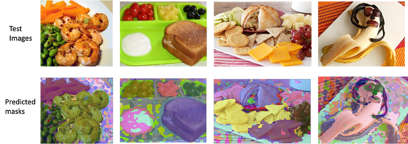
And here are randomly selected results, shown in Result figure 2.

Done 😃😃😃😃😃
Please feel free to take a look at the updated colab Notebook link: https://colab.research.google.com/drive/1UMQj7F_x0fSy_gevlTZ9zLYn7b02kTqi?usp=sharing
References
DINOv2: Learning Robust Visual Features without Supervision: https://arxiv.org/abs/2304.07193
If you like this work, then please share it with your friends like and follow me here on medium


