K-means Clustering: Intro with Math and Python

K-Means Clustering is one of the first algorithms I used in machine learning. During my Master's degree, one of my seniors asked me to help him with clustering because he knew I was into machine learning. I searched on the internet and found out about the K-Means algorithm. By searching more, I found a couple more articles—some had math, some used Python, and some had visualizations. So I thought about writing a complete post about k means using python and math introduction.

This article will walk you through the implementation of K-Means clustering in Python using a dataset of customer spending behavior. It will also explain the concepts behind it to help you understand how the algorithm works.

What is K-Means Clustering?

K-Means clustering is an algorithm that groups data into K distinct clusters based on their features. It works iteratively to assign data points to one of K clusters, minimizing the variance within each cluster. Each cluster is represented by its centroid, and the goal is to minimize the distance between the data points and their respective cluster centroids.

Mathematical Introduction to K-Means Clustering

K-Means clustering is an algorithm that partitions a dataset into K distinct clusters. The objective of K-Means is to minimize the variance within each cluster, which can be thought of as minimizing the distance between points within the same cluster and their cluster centroids. Here's a simple mathematical breakdown of the K-Means algorithm:

Initialization

We start with K random initial centroids, denoted as C₁, C₂, ..., Cₖ. These centroids can be selected either randomly or by using more sophisticated techniques like k-means++ to improve.

Assigning Data Points to the Nearest Centroid

For each data point (xᵢ) in the dataset (X), we assign it to the closest centroid based on a distance metric (usually the Euclidean distance). Mathematically, for each point (xᵢ), we find the centroid (Cⱼ) such that:

Here, |xᵢ - Cⱼ| represents the Euclidean distance between the point (xᵢ) and the centroid (Cⱼ).

Updating Centroids

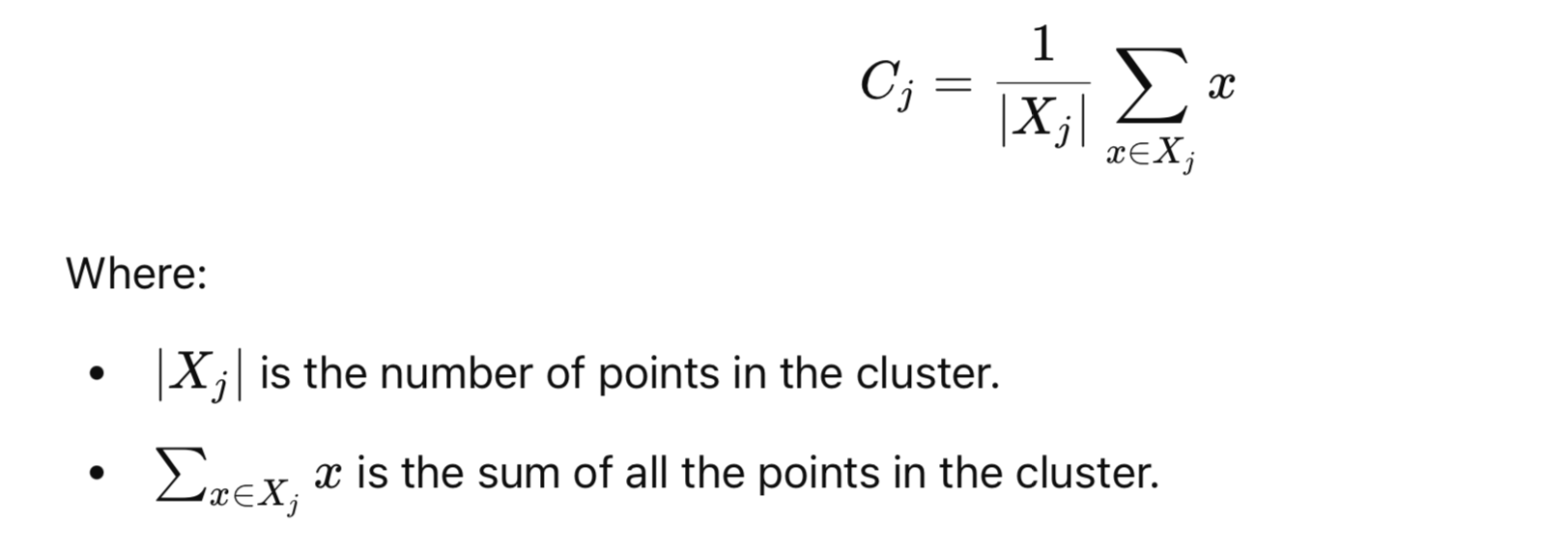
Once all data points have been assigned to clusters, we update the position of each centroid. The new position of a centroid is the mean of all the points assigned to it. If a centroid (Cⱼ) has been assigned a set of points (xⱼ), then the new centroid is calculated as:

Repeating the Process

Steps 2 and 3 are repeated iteratively until convergence, i.e., until the centroids stop moving or the change in centroids between iterations is below a certain threshold.

Objective Function: Minimizing the Within-Cluster Sum of Squares (WCSS)

The goal of K-Means is to minimize the Within-Cluster Sum of Squares (WCSS), which is the sum of the squared distances between each point and its assigned centroid. The WCSS is given by:

Minimizing WCSS ensures that the points within each cluster are as close to each other as possible, resulting in tighter and more defined clusters.

In summary, K-Means is an iterative algorithm that minimizes the sum of squared distances between points and their corresponding cluster centroids. It continues to update the centroids and reassign points until the solution converges, creating well-separated clusters.

Python Implementation

Let’s explore the step-by-step implementation.

Importing Libraries

The first step in implementing K-Means is importing the necessary libraries.

import numpy as np
import matplotlib.pyplot as plt
import pandas as pd

• Numpy: Provides support for numerical operations.
• Matplotlib: Used for plotting graphs.
• Pandas: Helps in data manipulation and analysis, particularly with structured data.

Importing the Dataset

At first download the dataset from below link.

We use a customer dataset that contains information about customers' annual income and spending score.

dataset = pd.read_csv('Mall_Customers.csv')
X = dataset.iloc[:, [3, 4]].values

• dataset: This is the DataFrame created by reading the CSV file.
• X: We extract the relevant columns (Annual Income and Spending Score) to perform clustering.

Using the Elbow Method to Find the Optimal Number of Clusters

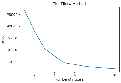
The elbow method helps determine the optimal number of clusters by plotting the Within-Cluster Sum of Squares (WCSS) against the number of clusters.

from sklearn.cluster import KMeans
wcss = []
for i in range(1, 11):
    kmeans = KMeans(n_clusters=i, init='k-means++', random_state=42)
    kmeans.fit(X)
    wcss.append(kmeans.inertia_)
plt.plot(range(1, 11), wcss)
plt.title('The Elbow Method')
plt.xlabel('Number of clusters')
plt.ylabel('WCSS')
plt.show()

Here’s what the code does:

• We import the KMeans class from scikit-learn.
• We initialize an empty list wcss to store the within-cluster sum of squares for each number of clusters.
• We use a for loop to run K-Means with n_clusters ranging from 1 to 10 and store the inertia_ (the sum of squared distances to the nearest cluster center) in wcss.
• The plot shows the elbow, which indicates the optimal number of clusters, in this case ir .

Training the K-Means Model on the Dataset

Once the optimal number of clusters (5 in this case) is determined from the elbow plot, we train the K-Means model.

kmeans = KMeans(n_clusters=5, init='k-means++', random_state=42)
y_kmeans = kmeans.fit_predict(X)

• kmeans: The KMeans model is initialized with 5 clusters and the k-means++ initialization method, which speeds up convergence.
• y_kmeans: This variable holds the predicted cluster for each data point.

Visualizing the Clusters

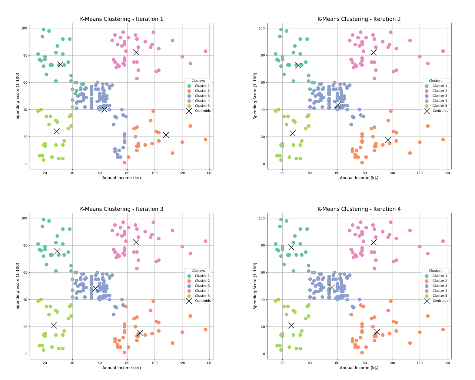
We can visualize the clusters to understand how the data is divided.

# Training in multiple steps and storing frames
frames = []
for i in range(1, 5):
    # Incrementally fit the model
    kmeans = KMeans(n_clusters=n_clusters, max_iter=i, init='k-means++', random_state=1, n_init=1)
    y_kmeans = kmeans.fit_predict(X)

    # Plotting the clusters
    plt.figure(figsize=(10, 8))
    colors = sns.color_palette("Set2", n_clusters)
    
    for j in range(n_clusters):
        plt.scatter(X[y_kmeans == j, 0], X[y_kmeans == j, 1], 
                    s=100, color=colors[j], label=f'Cluster {j+1}')
    
    # Marking the centroids
    plt.scatter(kmeans.cluster_centers_[:, 0], kmeans.cluster_centers_[:, 1], 
                s=300, c='black', label='Centroids', marker='x')
    
    # Adding plot title and labels
    plt.title(f'K-Means Clustering - Iteration {i}', fontsize=16)
    plt.xlabel('Annual Income (k$)', fontsize=12)
    plt.ylabel('Spending Score (1-100)', fontsize=12)
    plt.legend(title="Clusters", fontsize=10)
    plt.grid(True)

    # Save the current frame
    frame_path = f'{output_dir}/frame_{i}.png'
    plt.savefig(frame_path)
    plt.close()  # Close plot to prevent overlapping
    frames.append(frame_path)

# Create GIF from the saved frames
images = []
for frame in frames:
    images.append(imageio.imread(frame))

# Save the GIF
gif_path = 'kmeans_training.gif'
imageio.mimsave(gif_path, images, fps=1)

print(f"GIF saved successfully as {gif_path}")

• plt.scatter: We plot the data points for each cluster using a different color and label.
• kmeans.cluster_centers_: The cluster centroids are highlighted in yellow.
• The resulting plot visualizes how the customers are grouped into five distinct clusters based on their annual income and spending score.

Conclusion

In this implementation, we successfully used K-Means clustering to segment customers based on their annual income and spending score. This method is highly effective for customer segmentation in business applications, allowing businesses to understand and cater to different groups of customers more efficiently.

Your comments are valuable for me so please comment and share with your friends.

See you soon 😄